You need to understand mean reversion during this market downturn

It’s funny: a surprising number of investors don’t understand mean reversion. Even if you do, keep reading. I promise you’ll find this fascinating.

In finance or investing, mean reversion suggests that asset price volatility and historical returns eventually will revert to the long-run mean or average level of the entire dataset. 

Put another way: after a spectacular rise (like the one we just had), markets tend to “mean revert” back to more normal (i.e. lower) levels of pricing.

The chart below tracks 37 years of home price data – from January 1987 to August 2022 — for the three largest housing markets in California…

San Diego
Los Angeles
San Francisco

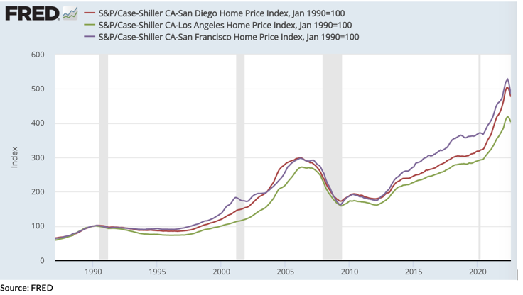
Booms and busts create peaks and valleys, as we all know. And if you want to know what kind of valley you might get after a recent peak, it’s worth looking at past valleys. The idea is to run a linear regression, not for the whole home-price data set, but just for the low points.

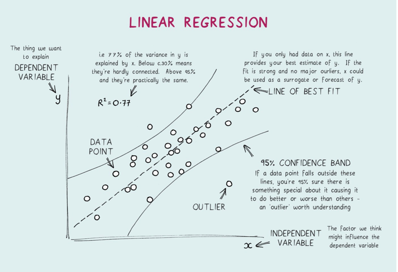
What we’ll end up with is called a “line of best fit,” that cuts through the scatterplot and shows us the trendline and the timing of historical valleys. In other words, a Price Reversion Trend Line.

See, once we know the trend of past valleys — and we adjust for inflation — we can project that line out into the future, and get a ballpark estimate of what the downside risk is in advance.

Based on this methodology, the future price reversion trendline suggests some big drops in California.

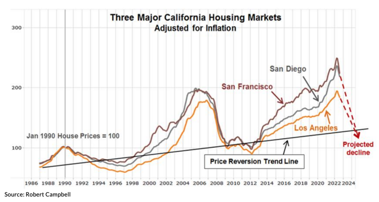
In fact, it’s statistically possible that SD, SF and LA — along with the rest of California — could see price drops of between 40%-50%.

In terms of the timing, the current down-cycle would take about 6 years to play out…which is in line with past valleys.

The U.S. housing cycles become far more apparent, because the data goes further back.

This informs us as to how U.S. housing cycles – like CA housing cycles – repeat over time and have a steady rhythm to them.

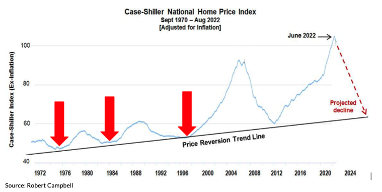
The chart below shows the peaks and valleys of U.S. inflation-adjusted home prices from September 1971 to August 2022.

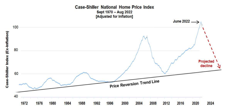
In the last 4 housing busts, home prices have fallen to somewhere between 50 and 60 on this index. Which is a fairly tight range.

And it’s interesting… it doesn’t seem to matter where the PEAK was. Home prices have still landed in that 50-60 range during a bust, though it’s been trending higher over time.

The point is, prices have reliably fallen into a range that is moving very gradually up and to the right. When we project that trend line into the future, you can see how far inflation-adjusted U.S. home prices could fall — around 40% — before they find price support once the bust cycle is over.

You may be thinking, “Dave, the only reason that prices dropped into that 50-60 range during the GFC is because of all the no-doc, stated income loans and ARMs. If it weren’t for that, prices would have eased down, and the valley would have been much more shallow, like in the 3 previous cycles.”

Fair enough. But if that can be said about the FALL in prices, can’t we say the same thing about the RISE in prices?

Meaning, if it weren’t for the availability of stated-income, no-doc loans and ARMs during the last cycle, prices wouldn’t have RISEN so high in the first place.

This is what people often forget. It wasn’t just the ultimate glut of supply that had “inorganic” roots. Demand was inorganic to begin with, thanks to artificial affordability.

If you think back to the run-up to the GFC, ARMs served as an affordability vehicle when interest rates rose…a vehicle that we haven’t had during this cycle.

Lending guidelines are more responsible, and borrowers have to qualify at the interest rate the ARM will ultimately adjust to, not the low teaser rate.

But what DID we have this time? Answer: the lowest interest rates in HISTORY

And aren’t low interest rates simply another affordability vehicle? One that, like ARMs, led to insane, “unnatural” demand and an overheated market?

Sure, those 3% loans aren’t going to adjust to a point where the borrowers can’t make their payment. That and high average home equity will help avoid the supply shock of a flood of foreclosures.

But in my opinion, they’ve had a very similar effect on demand.

I don’t think this cycle is THAT much different from the last. Both had an unnatural (artificial) affordability vehicle that created a frenzy… a frenzy to wildly overpay compared to intrinsic value.

Which leads you and I to at least have to consider the notion that this correction could be comparable to the last one.

I know I’m definitely in the minority here. Others aren’t even considering this. Everyone is telling you about…

All the home equity, and the high lending standards.

The low supply we have, and that we are underbuilt in the U.S.

And that, because more people can’t afford to buy, they’ll rent. And that’s true. We are definitely moving toward a renter nation.

Unless they can’t afford to rent. Then rents have to adjust. NOI goes down. Cap-rate compression turns to cap-rate expansion. There’s likely to be a fair bit of that ahead.